Any file, read accurately. 94.5% on real-world scans and photos.
| params | dimension | n heads | n layers | learning rate |
| 6.7B | 4096 | 32 | 32 | 3.0e-4 |
| 13.0B | 5120 | 40 | 40 | 3.0e-4 |
| 32.5B | 6656 | 52 | 60 | 1.5e-4 |
| 65.2B | 8192 | 64 | 80 | 1.5e-4 |
| params | dimension | n heads | n layers | learning rate |
| 6.7B | 4096 | 32 | 32 | 3.0e-4 |
| 13.0B | 5120 | 40 | 40 | 3.0e-4 |
| 32.5B | 6656 | 52 | 60 | 1.5e-4 |
| 65.2B | 8192 | 64 | 80 | 1.5e-4 |
Swipe up to continue
Reads the real world. Scanned, warped, photographed off a screen, unevenly lit or skewed: pages come out straight and structured.
Reads the real world. Skewed, photographed or off a screen, it comes back straight.
Revenue by region
Unaudited figures for the quarter ended 30 September 2026
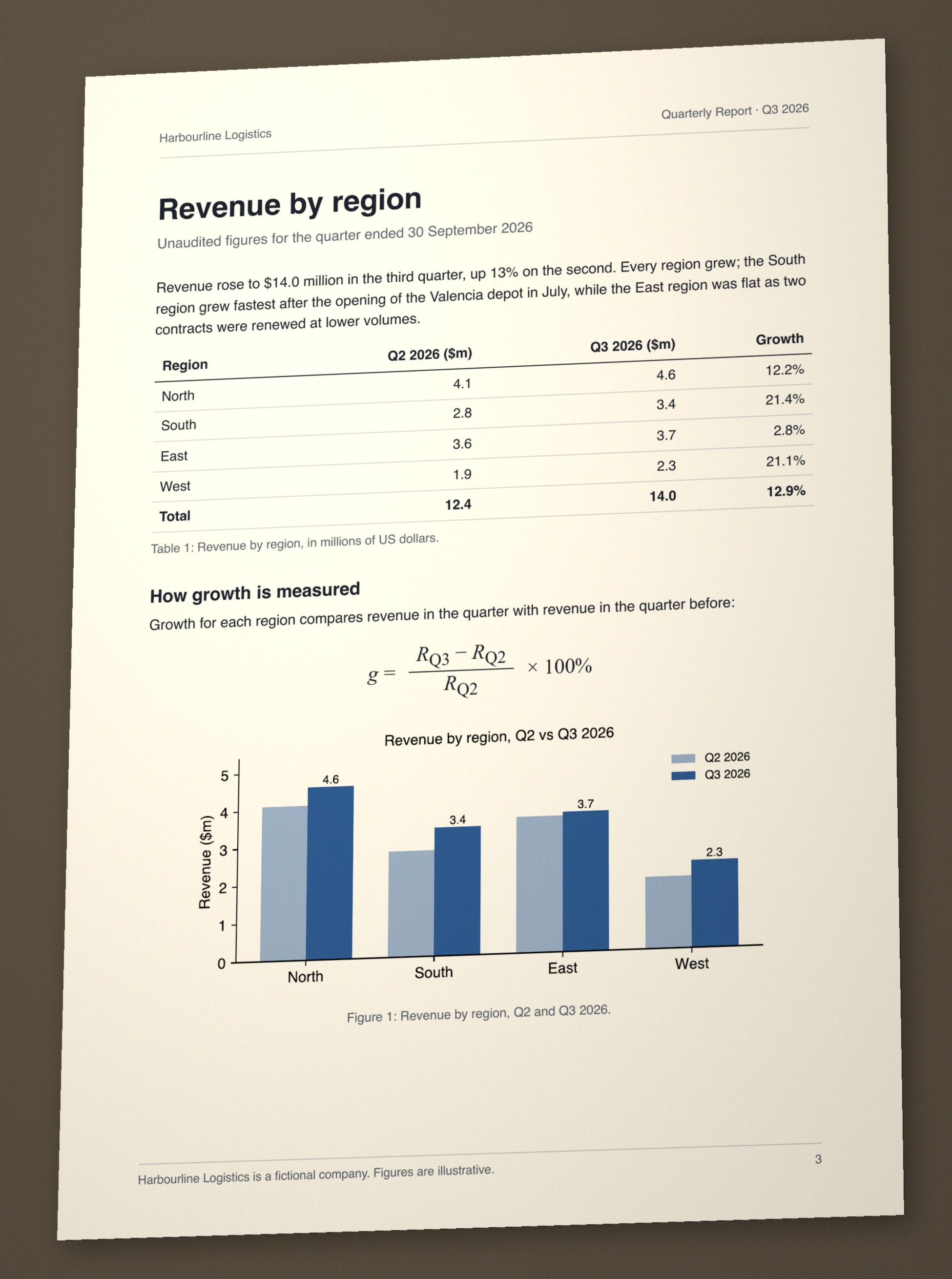
Revenue rose to $14.0 million in the third quarter, up 13% on the second. Every region grew; the South region grew fastest after the opening of the Valencia depot in July, while the East region was flat as two contracts were renewed at lower volumes.
| Region | Q2 2026 ($m) | Q3 2026 ($m) | Growth |
|---|---|---|---|
| North | 4.1 | 4.6 | 12.2% |
| South | 2.8 | 3.4 | 21.4% |
| East | 3.6 | 3.7 | 2.8% |
| West | 1.9 | 2.3 | 21.1% |
| Total | 12.4 | 14.0 | 12.9% |
Table 1: Revenue by region, in millions of US dollars.
How growth is measured
Growth for each region compares revenue in the quarter with revenue in the quarter before:
chart A grouped bar chart titled "Revenue by region, Q2 vs Q3 2026" compares revenue in $m across four regions.
Figure 1: Revenue by region, Q2 and Q3 2026.
Revenue by region
Unaudited figures for the quarter ended 30 September 2026
Revenue rose to $14.0 million in the third quarter, up 13% on the second. Every region grew; the South region grew fastest after the opening of the Valencia depot in July, while the East region was flat as two contracts were renewed at lower volumes.
| Region | Q2 2026 ($m) | Q3 2026 ($m) | Growth |
|---|---|---|---|
| North | 4.1 | 4.6 | 12.2% |
| South | 2.8 | 3.4 | 21.4% |
| East | 3.6 | 3.7 | 2.8% |
| West | 1.9 | 2.3 | 21.1% |
| Total | 12.4 | 14.0 | 12.9% |
Table 1: Revenue by region, in millions of US dollars.
How growth is measured
Growth for each region compares revenue in the quarter with revenue in the quarter before:
chart A grouped bar chart titled "Revenue by region, Q2 vs Q3 2026" compares revenue in $m across four regions.
Figure 1: Revenue by region, Q2 and Q3 2026.
Swipe up to continue
Formulas, read as math. Equations come back as clean LaTeX you can render, search and reuse.
Formulas, exactly. Printed or handwritten, back as clean LaTeX.
\[g=\frac{R_{Q3}-R_{Q2}}{R_{Q2}}\times100\%\]\[g=\frac{R_{Q3}-R_{Q2}}{R_{Q2}}\times100\%\]Swipe up to continue
Tables keep their shape. Merged cells, spanning headers and nested rows survive as real table structure, not flattened text.
Tables that stay tables. Merged headers survive, as a grid, HTML or JSON.
| params | dimension | n heads | n layers | learning rate | batch size | n tokens |
|---|---|---|---|---|---|---|
| 6.7B | 4096 | 32 | 32 | 3.0e-4 | 4M | 1.0T |
| 13.0B | 5120 | 40 | 40 | 3.0e-4 | 4M | 1.0T |
| 32.5B | 6656 | 52 | 60 | 1.5e-4 | 4M | 1.4T |
| 65.2B | 8192 | 64 | 80 | 1.5e-4 | 4M | 1.4T |
| params | dimension | n heads | n layers | learning rate | batch size | n tokens |
|---|---|---|---|---|---|---|
| 6.7B | 4096 | 32 | 32 | 3.0e-4 | 4M | 1.0T |
| 13.0B | 5120 | 40 | 40 | 3.0e-4 | 4M | 1.0T |
| 32.5B | 6656 | 52 | 60 | 1.5e-4 | 4M | 1.4T |
| 65.2B | 8192 | 64 | 80 | 1.5e-4 | 4M | 1.4T |
Swipe up to continue
Every block knows where it came from. Each piece of text carries a record of the page region it was read from: the first link in every answer’s trace.
Every block knows its source. The first link in every answer’s trace.
Hover a block on the page to see its record.
Hover a block on the page to see its record.
Swipe up to continue
More about Reader. Benchmarks, the pipeline and the output, in detail.
Swipe up to continue
Built for production
Built for production. What it takes to run it for real.
Figure text is read, never invented
Labels and captions in charts come from the image itself.
0 200 400 600 800 1000 1200 1400 Billion of tokens 1.5 1.6 1.7 1.8 1.9 2.0 2.1 2.2 Training loss LLaMA 7B LLaMA 13B LLaMA 33B LLaMA 65B
Results stream as pages are read
Each page is returned the moment it is done.
The whole engine on one GPU
Runs inside your perimeter, close to your data. Layout, OCR and orchestration share one GPU.
GPU
Layout
Regions and reading order
OCR
Text, tables and formulas
Orchestration
Straightens pages, routes each block
Measured, not promised. Every benchmark we ran.
Measured, not promised. Every benchmark we ran.
| Benchmark | AiQL Reader | OpenAI [MODEL NAME] | Google [MODEL NAME] | Anthropic [MODEL NAME] | xAI [MODEL NAME] |
|---|---|---|---|---|---|
| Real5-OmniDocBench Real-world capture, average of 5 conditions | 94.48% | [SCORE] | [SCORE] | [SCORE] | [SCORE] |
| OmniDocBench Overall, clean documents | 95.74% | [SCORE] | [SCORE] | [SCORE] | [SCORE] |
| OmniDocBench Formulas | 97.85% | [SCORE] | [SCORE] | [SCORE] | [SCORE] |
| olmOCR-bench Overall pass rate | 82.5% | [SCORE] | [SCORE] | [SCORE] | [SCORE] |
Real5-OmniDocBench
Real-world capture, average of 5 conditions
OmniDocBench
Overall, clean documents
OmniDocBench
Formulas
olmOCR-bench
Overall pass rate
How it reads every file. Each type takes the route built for it.
How it reads every file. Each type takes its own path to the same blocks.
PDF, Office, images, spreadsheets, web pages, audio, video and archives. Every file type in the docs →
Your fileHow it is readWhat comes back
Page reading
Straightened, laid out, then text from the file where it can be trusted and OCR otherwise
Tables
Sheet by sheet, cells, formats and merged headers kept
Markdown
Main content of a page, split text, code blocks
Timed segments
Speech transcribed; on-screen text read for video
Archives: every file inside goes the same way, up to 5,000 files, 4 GB, nested 4 deep.
Blocks
Each with its kind, content and where it came from.
What you get back. Choose the format per request.
What you get back. The same blocks, in the format you need.
ndjson
One line describes the document, then one line per page the moment that page is read, and a final line with time, usage and cost.
{"type":"document","version":1,"uid":"doc_46adfe42e230","title":"llama-page3","name":"llama-page3.pdf","format":"pdf","kind":"paged","unit":"page"}
{"type":"page","index":1,"size":[1447,2047],"markdown":"| params | dimension | n heads | n layer…","tokens":1207,"blocks":[{"id":"p1e1","kind":"table","label":"table","bbox":[276.506103515625,174.22686767578125,1169.7548828125,362.0890197753906],"polygon":[[276,174],[276,361],[1168,361],[1168,174]],"content":"| params | dimension | n heads | n layers | learning rate | batch size | n tokens |\n| --- | --- | --- | --- | --- | --- | --- |\n| 6.7B | 4096 | 32 | 32 | 3.0e-4 | 4M | 1.0T |\n| 13.0B | 5120 | 40 | 40 | 3.0e-4 | 4M | 1.0T |\n| 32.5B | 6656 | 52 | 60 | 1.5e-4 | 4M | 1.4T |\n| 65.2B | 8192 | 64 | 80 | 1.5e-4 | 4M | 1.4T |","tokens":175,"table":{"rows":[[{"text":"params","header":true},{"text":"dimension","header":true},{"text":"n heads","header":true},{"text":"n layers","header":true},{"text":"learning rate","header":true},{"text":"batch size","header":true},{"text":"n tokens","header":true}],[{"text":"6.7B"},{"text":"4096"},{"text":"32"},{"text":"32"},{"text":"3.0e-4"},{"text":"4M"},{"text":"1.0T"}],[{"text":"13.0B"},{"text":"5120"},{"text":"40"},{"text":"40"},{"text":"3.0e-4"},{"text":"4M"},{"text":"1.0T"}],[{"text":"32.5B"},{"text":"6656"},{"text":"52"},{"text":"60"},{"text":"1.5e-4"},{"text":"4M"},{"text":"1.4T"}],[{"text":"65.2B"},{"text":"8192"},{"text":"64"},{"text":"80"},{"text":"1.5e-4"},{"text":"4M"},{"text":"1.4T"}]]}}]}
{"type":"done","pages":1,"seconds":107.713147167,"cost":0.033948444805555554,"source":{"ocr_dpi":400}}markdown
The whole file as one Markdown document: headings, paragraphs and tables in reading order, formulas in LaTeX.
<!-- page 1 -->
| params | dimension | n heads | n layers | learning rate | batch size | n tokens |
| --- | --- | --- | --- | --- | --- | --- |
| 6.7B | 4096 | 32 | 32 | 3.0e-4 | 4M | 1.0T |
| 13.0B | 5120 | 40 | 40 | 3.0e-4 | 4M | 1.0T |
| 32.5B | 6656 | 52 | 60 | 1.5e-4 | 4M | 1.4T |
| 65.2B | 8192 | 64 | 80 | 1.5e-4 | 4M | 1.4T |
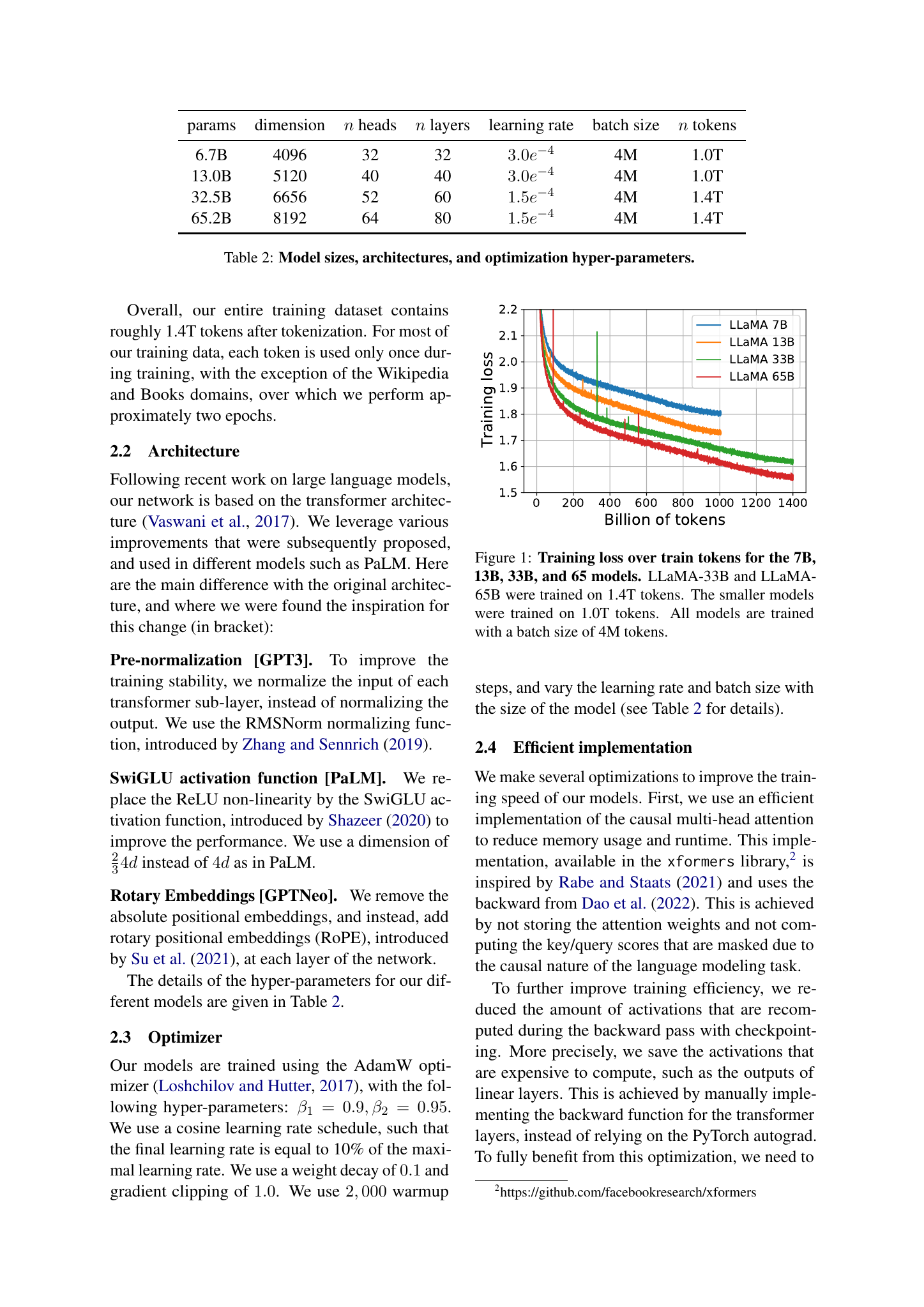
Table 2: Model sizes, architectures, and optimization hyper-parameters.
Overall, our entire training dataset contains roughly 1.4T tokens after tokenization. For most of our training data, each token is used only once during training, with the exception of the Wikipedia and Books domains, over which we perform approximately two epochs.
## 2.2 Architecture
Following recent work on large language models, our network is based on the transformer architecture (Vaswani et al., 2017). We leverage various improvements that were subsequently proposed, and used in different models such as PaLM. Here are the main difference with the original architecture, and where we were found the inspiration for this change (in bracket):
Pre-normalization [GPT3]. To improve the training stability, we normalize the input of each transformer sub-layer, instead of normalizing the output. We use the RMSNorm normalizing function, introduced by Zhang and Sennrich (2019).
SwiGLU activation function [PaLM]. We replace the ReLU non-linearity by the SwiGLU activation function, introduced by Shazeer (2020) to improve the performance. We use a dimension of \(\frac{2}{3}d\) instead of 4d as in PaLM.
Rotary Embeddings [GPTNeo]. We remove the absolute positional embeddings, and instead, add rotary positional embeddings (RoPE), introduced by Su et al. (2021), at each layer of the network.
The details of the hyper-parameters for our different models are given in Table 2.
## 2.3 Optimizer
Our models are trained using the AdamW optimizer (Loshchilov and Hutter, 2017), with the following hyper-parameters: \(\beta_{1} = 0.9\), \(\beta_{2} = 0.95\). We use a cosine learning rate schedule, such that the final learning rate is equal to 10% of the maximal learning rate. We use a weight decay of 0.1 and gradient clipping of 1.0. We use 2,000 warmup
A line chart titled by its axis labels plots Training loss against Billion of tokens for four LLaMA model sizes. The x-axis runs from 0 to 1400 in steps of 200; the y-axis runs from 1.5 to 2.2 in steps of 0.1. Four noisy, downward-curving series are shown: LLaMA 7B (blue) ends near 1.80 at 1000 tokens, LLaMA 13B (orange) near 1.73 at 1000, LLaMA 33B (green) near 1.61 at 1400, and LLaMA 65B (red) near 1.56 at 1400. Loss falls steeply at first and then flattens, and larger models reach lower loss at every token count. Short vertical spikes appear on the curves, most visibly a tall green spike near 330 tokens.
Text in the figure:
0 200 400 600 800 1000 1200 1400 Billion of tokens 1.5 1.6 1.7 1.8 1.9 2.0 2.1 2.2 Training loss LLaMA 7B LLaMA 13B LLaMA 33B LLaMA 65B
Figure 1: Training loss over train tokens for the 7B, 13B, 33B, and 65 models. LLaMA-33B and LLaMA- 65B were trained on 1.4T tokens. The smaller models were trained on 1.0T tokens. All models are trained with a batch size of 4M tokens.
steps, and vary the learning rate and batch size with the size of the model (see Table 2 for details).
## 2.4 Efficient implementationjson
The whole file as one JSON document, with every page and every block and its fields.
{
"document": {
"version": 1,
"uid": "doc_46adfe42e230",
"title": "llama-page3",
"name": "llama-page3.pdf",
"format": "pdf",
"kind": "paged",
"unit": "page"
},
"pages": [
{
"index": 1,
"size": [
1447,
2047
],
"markdown": "| params | dimension | n heads | n layers | learning rate | batch size | n tokens |\n| --- | --- | --- | --- | --- | --- | --- |\n| 6.7B | 4096 | 32 | 32 | 3.0e-4 | 4M | 1.0T |\n| 13.0B | 5120 | 40 | 40 | 3.0e-4 | 4M | 1.0T |\n| 32.5B | 6656 | 52 | 60 | 1.5e-4 | 4M | 1.4T |\n| 65.2B | 8192 | 64 | 80 | 1.5e-4 | 4M | 1.4T |\n\nTable 2: Model sizes, architectures, and optimization hyper-parameters.\n\nOverall, our entire training dataset contains roughly 1.4T tokens after tokenization. For most of our training data, each token is used only once during training, with the exception of the Wikipedia and Books domains, over which we perform approximately two epochs.\n\n## 2.2 Architecture\n\nFollowing recent work on large language models, our network is based on the transformer architecture (Vaswani et al., 2017). We leverage various improvements that were subsequently proposed, and used in different models such as PaLM. Here are the main difference with the original architecture, and where we were found the inspiration for this change (in bracket):\n\nPre-normalization [GPT3]. To improve the training stability, we normalize the input of each transformer sub-layer, instead of normalizing the output. We use the RMSNorm normalizing function, introduced by Zhang and Sennrich (2019).\n\nSwiGLU activation function [PaLM]. We replace the ReLU non-linearity by the SwiGLU activation function, introduced by Shazeer (2020) to improve the performance. We use a dimension of \\(\\frac{2}{3}d\\) instead of 4d as in PaLM.\n\nRotary Embeddings [GPTNeo]. We remove the absolute positional embeddings, and instead, add rotary positional embeddings (RoPE), introduced by Su et al. (2021), at each layer of the network.\n\nThe details of the hyper-parameters for our different models are given in Table 2.\n\n## 2.3 Optimizer\n\nOur models are trained using the AdamW optimizer (Loshchilov and Hutter, 2017), with the following hyper-parameters: \\(\\beta_{1} = 0.9\\), \\(\\beta_{2} = 0.95\\). We use a cosine learning rate schedule, such that the final learning rate is equal to 10% of the maximal learning rate. We use a weight decay of 0.1 and gradient clipping of 1.0. We use 2,000 warmup\n\nA line chart titled by its axis labels plots Training loss against Billion of tokens for four LLaMA model sizes. The x-axis runs from 0 to 1400 in steps of 200; the y-axis runs from 1.5 to 2.2 in steps of 0.1. Four noisy, downward-curving series are shown: LLaMA 7B (blue) ends near 1.80 at 1000 tokens, LLaMA 13B (orange) near 1.73 at 1000, LLaMA 33B (green) near 1.61 at 1400, and LLaMA 65B (red) near 1.56 at 1400. Loss falls steeply at first and then flattens, and larger models reach lower loss at every token count. Short vertical spikes appear on the curves, most visibly a tall green spike near 330 tokens.\n\nText in the figure:\n0 200 400 600 800 1000 1200 1400 Billion of tokens 1.5 1.6 1.7 1.8 1.9 2.0 2.1 2.2 Training loss LLaMA 7B LLaMA 13B LLaMA 33B LLaMA 65B\n\nFigure 1: Training loss over train tokens for the 7B, 13B, 33B, and 65 models. LLaMA-33B and LLaMA- 65B were trained on 1.4T tokens. The smaller models were trained on 1.0T tokens. All models are trained with a batch size of 4M tokens.\n\nsteps, and vary the learning rate and batch size with the size of the model (see Table 2 for details).\n\n## 2.4 Efficient implementation\n\nWe make several optimizations to improve the training speed of our models. First, we use an efficient implementation of the causal multi-head attention to reduce memory usage and runtime. This implementation, available in the xformers library,<sup>2</sup> is inspired by Rabe and Staats (2021) and uses the backward from Dao et al. (2022). This is achieved by not storing the attention weights and not computing the key/query scores that are masked due to the causal nature of the language modeling task.\n\nTo further improve training efficiency, we reduced the amount of activations that are recomputed during the backward pass with checkpointing. More precisely, we save the activations that are expensive to compute, such as the outputs of linear layers. This is achieved by manually implementing the backward function for the transformer layers, instead of relying on the PyTorch autograd. To fully benefit from this optimization, we need to\n\n<sup>2</sup>https://github.com/facebookresearch/xformers",
"tokens": 1207,
"blocks": [
{
"id": "p1e1",
"kind": "table",
"label": "table",
"bbox": [
276.506103515625,
174.22686767578125,
1169.7548828125,
362.0890197753906
],
"polygon": [
[
276,
174
],
[
276,
361
],
[
1168,
361
],
[
1168,
174
]
],
"content": "| params | dimension | n heads | n layers | learning rate | batch size | n tokens |\n| --- | --- | --- | --- | --- | --- | --- |\n| 6.7B | 4096 | 32 | 32 | 3.0e-4 | 4M | 1.0T |\n| 13.0B | 5120 | 40 | 40 | 3.0e-4 | 4M | 1.0T |\n| 32.5B | 6656 | 52 | 60 | 1.5e-4 | 4M | 1.4T |\n| 65.2B | 8192 | 64 | 80 | 1.5e-4 | 4M | 1.4T |",
"tokens": 175,
"table": {
"rows": [
[
{
"text": "params",
"header": true
},
{
"text": "dimension",
"header": trueEvery block, fully described. Each page carries its Markdown, size and a list of blocks like this one.
{
"id": "p1e1",
"kind": "table",
"label": "table",
"bbox": [
276.506103515625,
174.22686767578125,
1169.7548828125,
362.0890197753906
],
"polygon": [
[
276,
174
],
[
276,
361
],
[
1168,
361
],
[
1168,
174
]
],
"content": "| params | dimension | n heads | n layers | learning rate | batch size | n tokens |\n| --- | --- | --- | --- | --- | --- | --- |\n| 6.7B | 4096 | 32 | 32 | 3.0e-4 | 4M | 1.0T |\n| 13.0B | 5120 | 40 | 40 | 3.0e-4 | 4M | 1.0T |\n| 32.5B | 6656 | 52 | 60 | 1.5e-4 | 4M | 1.4T |\n| 65.2B | 8192 | 64 | 80 | 1.5e-4 | 4M | 1.4T |",
"tokens": 175,
"table": {
"rows": [
[
{
"text": "params",
"header": true
},
{
"text": "dimension",
"header": true
},
{
"text": "n heads",
"header": true
},
{
"text": "n layers",
"header": true
},
{
"text": "learning rate",
"header": true
},
{
"text": "batch size",
"header": true
},
{
"text": "n tokens",
"header": true
}
],
[
{
"text": "6.7B"
},
{
"text": "4096"
},
{
"text": "32"
},
{
"text": "32"
},
{
"text": "3.0e-4"
},
{
"text": "4M"
},
{
"text": "1.0T"
}
],
…
]
}
}- id
- Page and position: p1e1 is the first block on page 1.
- kind
- heading, text, table, formula, figure, chart, caption, footnote, header, footer, page_number or other.
- label
- The layout model's own name for the region.
- level
- For headings: how deep in the outline.
- bbox
- Its box on the page, [x0, y0, x1, y1], in pixels of the page image.
- polygon
- Its outline when the region isn't an upright box, e.g. on a tilted photo.
- content
- The text: Markdown for tables, LaTeX for formulas, a description for figures.
- table
- For tables: rows of cells, with header cells and spans marked.
- time
- For audio and video: start and end in seconds.